Ontology of measurement, control, retunability, and stable law
0. Orientation
What kind of world can be known at all? Not only what happens, but what kind of structure makes repeatable facts, reliable prediction, and purposeful intervention possible?
Physics usually begins after a regularity has become visible. It asks what equations describe it, what symmetries preserve it, and what mechanisms produce it. The Continuum Computation Thesis (CCT) begins one step earlier. It asks what had to be physically true of the observer, instrument, estimator, and controller for that regularity to become stable enough to count as a fact.
No real observer sees everything. A telescope trades field of view for resolution. A detector has thresholds, dead time, and noise. An estimator carries assumptions about what should be averaged and what should be preserved. A controller acts through latency, finite bandwidth, imperfect commands, and a changing environment. Even the most abstract observer is eventually embodied in a physical chain that must receive, transform, store, and compare information.
CCT takes that chain seriously as part of the phenomenon. The system being studied still has its own dynamics, but the scientific object is larger than the isolated target. It includes the system, observer, instrument, estimator, drive, controller, environment, and the resources and support that allow the arrangement to operate. Change the arrangement and some regularities remain. Others sharpen, soften, move, or disappear. The pattern of those changes can itself become an object of physics.
We have inherited two vocabularies for describing change. Physics speaks in fields, forces, states, symmetries, and dynamics; computation speaks in transformation, memory, selection, error correction, and constrained information flow. CCT asks whether they are two coordinate systems for the same deeper process: connected physical evolution becoming legible and steerable through finite participation.
Here, continuum means connected physical dynamics. Computation means rule-governed transformation under constraints. The thesis places process before record: bits, clicks, traces, estimates, and commands are stable forms produced where a richer physical process meets a finite interface.
If measurement and control help determine which physical distinctions become usable, they become part of the architecture being designed rather than passive accessories to a finished experiment. A different readout, timing structure, field geometry, feedback loop, or estimator may make a regime visible that brute-force input leaves hidden. This practical expression is what CCT calls programmable physics.
CCT therefore studies the gap between physical possibility and physical access. Physical law bounds what can happen. The complete arrangement helps determine which lawful records, states, and transitions become observable, reachable, retainable, repeatable, and controllable for finite participants under real conditions.
The same premise opens a deeper possibility: perhaps the laws we know are exceptionally stable structures that finite observers can reconstruct across changes of representation, scale, and intervention, rather than only equations written against an external backdrop. That possibility has a life of its own in mathematics and theory, where it can generate models, theorems, counterexamples, equivalence questions, and accounts of stable law before a laboratory can touch its furthest implications.
That possibility begins from an established foundation. Quantum field theory contains observer-dependent particle descriptions. Quantum Darwinism studies how selected records become stable and redundantly accessible through an environment. Renormalization describes stable effective structure under changes of scale, and an information-geometric formulation makes operational distinguishability part of that flow. Operational reconstructions of quantum theory, quantum reference frames, and finite quantum clocks likewise show that access, reference, and physical resources can enter the structure of a description.
Each result belongs to its own mature theory. Layer 3 asks whether they are isolated domain facts or fragments of a more general relationship between finite observers and stable physical law. Recovering those results in one grammar, generating a theorem that their separation does not suggest, and extracting a prospective discriminator are three ways that question can become precise.
Current physics is the map CCT must recover, not the boundary of what CCT is allowed to ask.
Its empirical success is CCT's compulsory stability record. The ontology remains open: particles, constants, laws, and causal handles may be exceptionally persistent interfaces through which finite observers reconstruct a richer physical process.
The practical and theoretical paths meet in one idea: retunability. Operationally, it means moving a physical arrangement among stable effective regimes by changing measurement, timing, coupling, boundaries, feedback, or drive, a search that can proceed now inside established physics. Its ontological reach is wider, asking whether some structures treated as fixed within one description are stable settings of a larger rule-space and, in turn, what stable law itself might be.
1. The Mirage of the Digital-Physical Split
We often speak as if there were a digital world made of bits and a physical world made of matter and fields. Yet a bit is already a physical achievement. Voltages must cross thresholds. Clocks must coordinate transitions. Memory states must persist against noise. Error correction must keep one symbol distinguishable from another.
The reverse is also true. A physical process becomes scientifically usable only when some part of it can be rendered into a stable record. What looks like a division between two worlds is often a difference between process and report.
1.1 Instruments as compilers
An instrument is a physical translator. It exposes only a slice of what occurs, enforces a grammar for what can be recorded, and trades resolution, range, timing, and noise to produce a stable report. A camera compiles electromagnetic interaction into pixels. A particle counter compiles interaction into events. A phase-sensitive receiver compiles related dynamics into a continuous trace with a different error structure.
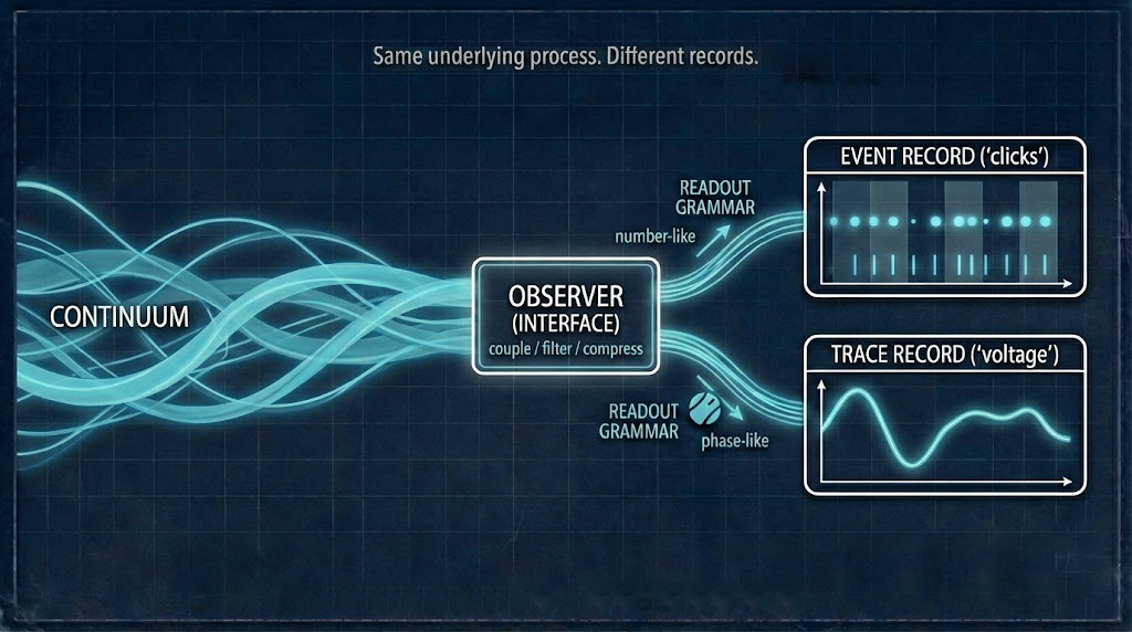
Calling instruments compilers shifts the emphasis. The record is neither a transparent copy of an object nor a free invention of an observer. It is a physically produced relation. The target, coupling, detector, timing, estimator, and storage chain jointly determine which distinctions survive long enough to be compared.
A familiar image makes this easier to hold. The ocean is not blue as an isolated property of water. Blue is what water, illumination, scattering, atmosphere, and a visual system make legible together. The colour is real as a stable relation, but its form belongs to the whole interaction.
Digital audio shows the same structure in engineering form. A microphone follows a continuous pressure wave. A converter samples it. Filters remove some frequencies and preserve others. Quantization maps amplitudes into finite levels. Storage and playback reconstruct a signal from that record. Change the chain and the audible world changes with it, even when the source is held fixed.
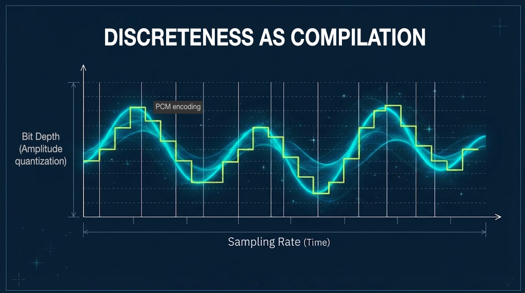
The underlying thought can be stated compactly:
The continuum is the connected process; discrete reports are what finite instruments can stabilize.
This statement opens an experimental question. Is a step, click, category, or apparent boundary invariant across measurement grammars? Does it belong to the target dynamics, the target-detector interaction, the readout architecture, or a relation shared across them? Once the complete chain is visible, those possibilities can be separated rather than collapsed into one word: measurement.
1.2 From record to mechanism
Thresholds turn smooth variation into events. Integration windows trade timing for precision. Phase references reveal relations that intensity-only measurements cannot. Estimators preserve some structures and average away others. These choices form a measurement grammar: the set of distinctions an experiment is physically able to write.
As the grammar changes, the report may change with it, making the invariants and the newly legible features the important objects of study. A change of detector or estimator is therefore a physical intervention in the experiment even when the target system is untouched.
If instruments translate connected dynamics into finite records, then computation begins within the act by which the world becomes available to a finite observer. The digital and the physical become two dialects of one recursive transformation.
The old split then gives way to a different set of questions. We move from states alone to transformations, from measurement as mirror to measurement as participation, and from control over a passive object to co-tuning with a responsive system. The physical situation becomes more complete.
2. The Continuum and Rule-Space
If process comes before report, what remains when we stop treating the report format as the ontology?
CCT begins with connected dynamics: a physical process unfolding through relations that may be continuous even when the records made from them are finite. "Continuum" names no hidden ether. It names the process under interaction, while our descriptions are the stable forms produced by bounded access to it.
Because a connected process can behave in many ways, the picture immediately raises another question: what determines the regime it inhabits?
CCT uses rule-space for the parameters, constraints, couplings, boundaries, equivalences, and validity domains that make one regime different from another. At the operational level, rule-space is the landscape that experimentalists and engineers already traverse. Temperature, geometry, phase, timing, gain, feedback, environment, drive waveform, estimator, and coarse-graining can all move a system through that landscape.
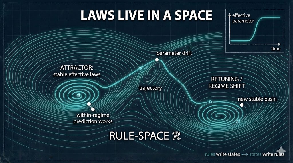
The landscape metaphor is useful because control is rarely a matter of adding more of one scalar input. A system may sit in a valley, protected from small disturbances. A ridge may separate two stable modes. A narrow pass may offer a low-cost transition that brute force misses. A route that reaches a state quickly may fail to hold it; another may preserve coherence but demand more calibration or timing support.
Rule-space changes the order of search. Instead of choosing one familiar operating point and explaining its output afterward, we can ask which intervention would most sharply separate candidate mechanisms, which region should be searched next, and which observer/controller arrangement would make the difference legible before the result is known.
At the deeper level, rule-space becomes an ontological conjecture. Perhaps the laws we know are exceptionally persistent regions in a wider space of possible descriptions and relations. Their empirical success then becomes the first great stability phenomenon the theory must explain. Why are quantum theory, relativity, and field theory so reconstructible across observers and regimes? What survives changes of coordinates, basis, scale, and measurement grammar? Which distinctions are physics, and which are only descriptions of physics?
Retuning makes this question geometric. If an instrument or controller changes, how is the "same" inferred quantity carried from one setting to another? One can picture the control settings as a base space, with effective descriptions attached to each point. Calibration supplies a transport rule. Move through a closed loop and the result may return unchanged, or it may carry drift, hysteresis, or path dependence. The loop reveals whether retuning was a clean re-description or whether the regime itself changed.
At the horizon of the theory, the same problem returns as the possibility that stable law is what survives transport through transformations that should leave the physics unchanged.
3. Information and Feedback: How Regimes Persist
A continuum of possible change is not yet a world of stable objects. Something must preserve distinctions long enough for structure to appear.
CCT treats information as relational constraint: the pattern that lets a system select, suppress, hold, recover, or distinguish possible states. A record is useful because it preserves a distinction. A controller is useful because it changes which outcomes remain reachable. Information is carried physically, maintained through timing and memory, and exposed to noise, drift, calibration error, and energetic cost.
Feedback is how those constraints become persistent structure.
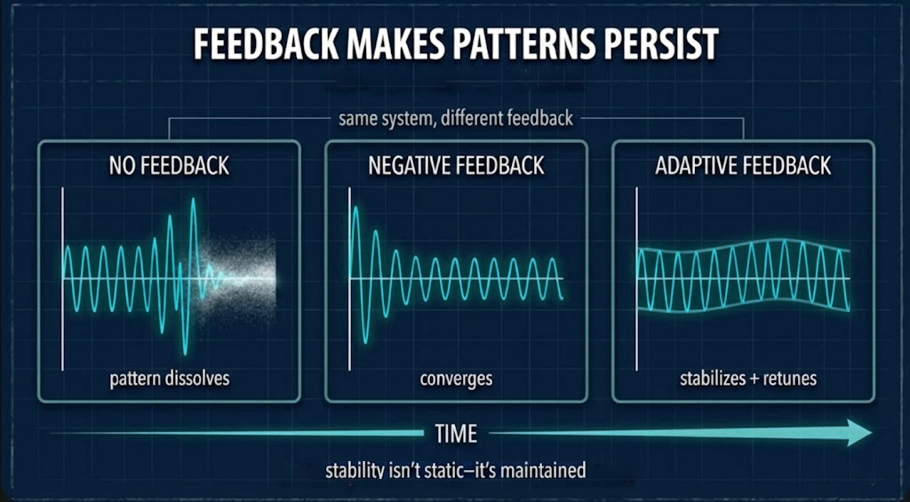
Damping suppresses motion. Gain amplifies selected differences. Delay can stabilize, destabilize, or synchronize. Coupling creates collective modes. Error correction preserves a relation against disturbance. Boundaries redirect flows. These moves recur often enough that CCT speaks of a feedback grammar.
The phrase invites comparison while a cavity, a material phase, a cell, and a control policy retain their different physical mechanisms. Each can still be asked a common family of questions. What distinction is being resolved? What pattern is being stabilized? What resource keeps it coherent? What changes when the observer or controller changes?
If that grammar transfers across domains, it should do more than produce a suggestive analogy. It should help select a discriminator prospectively. The common language earns value when it predicts which intervention, measurement, or operating region will separate alternatives under matched information and resources.
Feedback also gives law and novelty a way to coexist. Within a regime, a system may evolve deterministically, stochastically, or through a mixture of both. Yet the regime itself can change when boundaries, symmetries, relevant timescales, or couplings are reorganized. Bifurcations, phase transitions, renormalization flows, and adaptive systems all show familiar forms of lawful change in effective description.
CCT extends that intuition: creativity in nature may come from structured changes in the space of constraints. Rules write states; states alter the conditions under which the next rules act. Order persists, but it need not be frozen.
Nature may change its mind without breaking its laws.
Retunability remains constrained: you can change the game, but you still have to pay for the new board.
4. Programmability: The Measure of Lawful Steering
With feedback in place, a practical question emerges: how much can a physical arrangement be made to retune?
Although programmability is often spoken of as though it belonged to an object, in practice it belongs to a relation: a system is programmable for a task when an observer/controller arrangement can place, hold, distinguish, switch, or recover relevant states over a declared time and operating range.
That relation includes more than the command sent to the target. It includes what the controller can observe, what the actuator actually delivers, what the environment perturbs, and what support keeps the arrangement running. A control effect that depends on hidden cooling, repeated calibration, synchronized infrastructure, discarded trials, or an alternate information channel carries those dependencies with it.
CCT's operational gauge, \(\mathsf{Prog}_T\), asks how much task-relevant steering is achieved over horizon \(T\) under that complete boundary. Energy is a central physical cost, but it lives beside latency, calibration, synchronization, memory, setup, instability, reliability, failed attempts, and support burden.
These resources can sometimes be combined into a declared scalar comparison, while in other cases the scientific object is a resource front. One method may use less energy while another is faster, more selective, more reversible, or able to reach a state that the first cannot access; several legitimate leaders may remain because the tradeoff itself is the discovery.
Structured control can therefore matter even when it does not simply minimize joules. Timing, phase, geometry, feedback, or mode selection may buy access to a narrow regime, preserve a delicate state, or make a transition reliable, making brute force and orchestration different routes through rule-space rather than settings on one power dial.
Three kinds of coherence must be kept apart. Estimator coherence belongs to the measurement and inference chain. Drive coherence belongs to the timing, phase, waveform, or mode structure of the command. State coherence belongs to the physical system. A smoother record may come from a better estimator. A beautifully structured drive may leave the state unchanged. A coherent state may exist while remaining inaccessible to the declared controller. The distinctions tell us where the actual leverage lives.
The cross-domain programmability hypothesis can now be stated precisely. What may transfer is the shape of the question rather than one value or scaling law: finite observers and controllers encounter bandwidth, noise, back-action, timing, reliability, and resource tradeoffs in many substrates. The wager is that a common grammar can help find useful regimes across those differences.
A two-ring image captures the reach of the idea. The inner ring, where familiar physics holds the effective laws fixed while states, controls, and observer arrangements vary, contains most programmable-physics discovery. Around it lies an outer ring in which the stability and reconstruction of the effective laws themselves become the question. The familiar inner domain grounds that deeper inquiry into why it is so stable.
Programmability, in this sense, is a form of lawful creativity: the capacity to reorganize what a system can do while remaining inside the constraints that make the change coherent and real.
5. Observation as Participation
No observer stands outside the process. To measure is to couple, filter, integrate, threshold, estimate, and record. Observation is participation in a physical relation, even when the back-action is extremely small.
Quantum measurement makes this participation especially vivid. In a double-slit arrangement, propagation and interference are represented one way, while detection produces localized records. CCT reads the click as a stable record formed through interaction with a finite detector and readout chain, while a phase-sensitive or quadrature-like measurement can expose a different aspect of the same experimental situation.
The mechanism layer remains established quantum physics, including its quantized energy structure and successful predictions. CCT adds an observer-contract question: how do record form, estimator error, and accessible structure change as the physical measurement grammar changes?
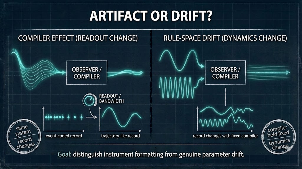
The Resolution Filter Hypothesis (RFH) is one way to make that question operational. It asks whether a declared error or discreteness measure changes systematically with effective measurement bandwidth. In one regime the relation may look smooth. In another it may show a knee, band structure, or a stable floor. The fitted behavior belongs to the whole observer-and-estimator contract; no universal exponent is assumed.
The philosophical point is larger than one scaling relation. Knowledge is not a mirror detached from the world. It is a stable relation achieved by a physical system capable of preserving distinctions, testing transformations, and correcting error. To model creates a feedback path between data, expectation, and intervention. To control tests whether an inferred structure has causal leverage.
Scientific objectivity becomes the search for what survives the changes that should leave the phenomenon intact: changes of observer, estimator, representation, and laboratory. Observation is participatory, but truth is not arbitrary. It is what remains after the relation has been varied, challenged, and reconstructed.
6. Stable Law, Time, and the Living Rule-Space
Beyond the operational question of how observers and controllers reveal effective regimes lies the philosophical question of why any regime remains stable and communicable across observers at all.
One possible answer is that a law is a highly persistent structure under reconstruction. Different finite observers may receive different records and still recover equivalent relations. Stable law would then be what survives the relevant changes of scale, representation, measurement grammar, and intervention.
The theory can therefore ask what counts as the same physical law under a change of coordinates or basis, what a finite observer can reconstruct from incomplete records, and whether a model derives why a particular pattern is special or merely expresses many possibilities. Across those questions runs a search for invariants that remain after the descriptive scaffolding has changed.
Time also looks different through this lens. Rather than appearing only as an external stage on which change occurs, time can be studied through the ordering and composability of physical updates: the rhythm by which one transformation becomes the condition for the next, and by which change becomes record.
Constants can be approached as exceptionally stable parameters of effective description, values that preserve coherent reconstruction across the regimes we inhabit. Understanding their persistence comes first, and a deeper account earns its place by explaining why familiar physical structures remain so difficult to dislodge and so easy to share among observers.
Here the theory becomes autonomous, able to advance through a theorem, a counterexample, a reconstruction result, a proof of equivalence, or a demonstration that an appealing signature is non-unique. A no-go result can be a genuine discovery because it permanently removes a false path through rule-space.
The world described here is therefore neither a machine with eternally fixed gears nor a flux without form. It is lawful enough to be known and open enough to generate new regimes. Stable law is the durable achievement; retunability is the structured possibility around it.
7. From Philosophy to Search
An ontology matters when it changes what becomes searchable.
CCT moves in two directions from the same source. Along the generative-theory path, the observer-conditioned picture becomes model classes, reconstruction maps, consistency conditions, theorems, counterexamples, and questions about stable law. These results have independent value: mathematics can close a seductive route, reveal a hidden equivalence, or show that a proposed structure is too expressive to be specific.
Along the programmable-physics and physical-access path, selected parts of the framework become questions about what can be made newly measurable, steerable, or decidable. Simulations construct estimators, map operating regions, and expose confounders; experiments vary measurement grammar, timing, coherence, feedback, geometry, and environmental handles. Competing approaches receive the same prior information and a comparable resource boundary so that prospective selection can be distinguished from explanation after the fact.
CCT Labs carries that second path through three movements. It Scouts widely enough to discover. It Discriminates by selecting the observation or intervention that most sharply separates alternatives. It Promotes what survives stronger accounting, uncertainty, reliability, and replication. Rigor enters with increasing force as the claim strengthens, while scouting remains open enough to find the unexpected.
A promoted operation can become a reusable physical-access primitive: a bounded way of making an observation, state, or transition available with known conditions, costs, and failure modes. CCT's first finite two-component composition contract and source-linked prospective atlas now make part of composition executable before physical exposure. The broader philosophical and engineering question is whether individually valid operations remain jointly possible in evidence-bearing systems, or whether their measurements, controls, environments, and resource demands change one another.
Selected Formal Results and Open Questions carries the public form of the first path. The two remain in conversation. Theory changes which regimes are worth searching. Simulation and experiment reveal which distinctions remain consequential. What survives returns as a new constraint on the theory.
Ontology expands the search space. Theory gives it form. Prediction selects where to look. Simulation explores candidate regimes. Physical exposure tests what survives. What survives can become a reusable primitive, a composition target, or a sharper theory.
Taken together, these movements form the full CCT arc: finite observers and complete arrangements open two connected searches, one toward resource-bounded physical access and composition, the other toward a theory of stable law. Progress need not wait for the furthest conjecture to be settled: a new theorem, a closed route, a better discriminator, a predicted operating region, a physical exposure, or a reusable capability can each change what the program is able to ask next.
The Guiding Horizon is active within that arc. Difficult application, infrastructure, and mission questions can work backward to generate present requirements without deciding in advance what the search will find. Tau-X is the flagship space-and-motion expression of that horizon, while sensing, materials, manufacturing, and field control provide nearer domains for the same physical-access logic.
8. A Compact Statement
Continuity is the physical process; finite observers stabilize records.
Measurement is compilation through a physical grammar.
Feedback turns constraint into persistence, transition, and recovery.
Rule-space maps the regimes a system and observer can jointly inhabit.
Programmability is reliable steering under the resources needed to perform the task.
Physical access is the lawful record, state, or transition a complete arrangement can make reliably available.
Retunability is lawful movement among stable regimes.
An access primitive preserves one such operation with its validity and cost; composition tests whether several operations remain valid together.
Stable law is what remains reconstructible across the changes that should leave the physics intact.
CCT therefore holds open two connected possibilities: a better practical way to discover, expose, retain, and compose useful physical access, and a more generative theoretical account of why particular regularities become stable for finite observers and controllers.
The possibility is unresolved. Its paths of thought, proof, simulation, and physical exposure are concrete.
For the conceptual derivation, continue to The First-Principles Path to CCT. For selected results and the possibilities they open, see What CCT Has Built and Opened. For the wider technical record, enter the Research Library.
CCT: A Plain-Language Philosophy of Measurement, Control, and Stable Law
The Question Behind CCT
Physics gives us extraordinarily successful descriptions of the world. It tells us how light bends, how matter changes phase, how particles interact, and how planets move. CCT begins with a quieter question:
How did those regularities become visible to us in the first place?
Every observer is limited. That includes people, but it also includes cameras, detectors, estimators, computers, and feedback systems. A sensor can only respond so quickly. A camera sees some wavelengths and misses others. A controller acts after a delay. An experiment has noise, drift, limited memory, and a finite amount of energy and time.
The Continuum Computation Thesis (CCT) treats those limits as part of the physical situation. Instead of imagining a perfect observer looking at a finished world from outside, it studies the whole arrangement: the target system, instrument, estimator, drive, controller, environment, and the support needed to make them work.
Change that arrangement and the world itself has not necessarily changed, but what becomes visible and controllable may change a great deal. A faint pattern can become measurable. A state that looked unstable can become easy to hold. A sharp boundary can soften into a gradual transition. A useful regime can appear where a brute-force search found nothing.
That is the practical promise of CCT. Its deeper question is more philosophical: perhaps what we call a stable law is connected to what finite observers can keep reconstructing across many different ways of measuring and acting.
Current physics is the best map of the stable regimes we already know, and every deeper account has to recover its success. CCT keeps open whether that map is also the final grammar of reality.
Physics already gives us pieces of this puzzle. Accelerating observers can disagree about particles. Environments can make some records stable and widely accessible. Coarse-graining can turn microscopic detail into durable large-scale laws. Finite clocks and reference frames limit which descriptions are available. CCT asks whether these are separate facts or signs of a more general relationship among observers, records, resources, and stable physical structure.
A map can be indispensable without being final.
The name joins those two ideas. Continuum means connected physical change. Computation means lawful transformation under constraints. CCT pictures the world as an ongoing physical process, while instruments and controllers turn parts of that process into records and actions they can preserve.
1. The World We Record
Imagine hearing a song through a wall. The bass passes through easily. The higher notes are muffled. You still hear the song, but you hear a version shaped by the wall, the room, your ears, and where you are standing.
A scientific instrument works in the same general way. It selectively translates a physical process into a form that can be stored and compared.
A camera turns light into pixels. A particle detector turns an interaction into a click. A microphone turns changing air pressure into an electrical signal. A computer turns changing voltages into stable bit patterns by enforcing thresholds and timing.
CCT calls an instrument a compiler because it gives the process a readable grammar. It decides which differences can survive into the record.
Think about digital audio. The pressure wave in the air changes continuously. A recorder samples it at particular moments, filters it, rounds the measurements, stores them, and later reconstructs a sound. Raise the sampling rate and some details return. Change the filter and others disappear. The source can stay fixed while the available world of the recording changes.
Colour gives another example. The ocean is not blue all by itself. Its colour comes from water, sunlight, scattering, atmosphere, and a visual system. Blue is real, but it is real as a stable relation among those things.
The recording-chain example leads to one of CCT's central images:
The continuum is the connected process; discrete reports are what finite instruments can stabilize.
A click, pixel, trace, or estimated state is therefore more than a fact about an isolated object. It is a fact produced through an interaction. The scientific question becomes richer: which part of the pattern belongs to the target, which part comes from the measurement chain, and which part remains stable across both?
Different instruments write different kinds of sentences about the world. A threshold produces a yes-or-no event. A long averaging window gives a precise value but loses timing detail. A phase-sensitive detector reveals relationships that an intensity-only detector cannot see. An estimator may preserve a slow trend while smoothing away rapid change.
Together these choices form a measurement grammar. Once we can vary that grammar deliberately, measurement becomes one of the experiment's design variables rather than only a report at its end.
2. A Landscape of Possible Regimes
Now imagine a ball resting in a landscape of hills and valleys. If it sits at the bottom of a deep valley, a small push will not move it very far. If it sits near a ridge, a tiny change may send it into a completely different valley.
The valleys are stable regimes. The ridges are boundaries. The paths between them are possible transitions.
CCT calls this landscape rule-space. At the practical level, it includes all the conditions that help a physical system behave one way rather than another: temperature, geometry, timing, coupling, feedback, field shape, drive waveform, environment, measurement method, and the way the result is estimated.
This changes how we think about control. The obvious approach is often to push harder by adding power, applying a larger field, or increasing the gain. Yet if the real problem is finding a narrow pass through the landscape, pushing harder in the wrong direction may do very little.
A carefully timed sequence may reach a state that a large constant input misses. A different detector may reveal that the state was present all along but hidden by the readout. A feedback loop may hold a regime that disappears under open-loop control. Geometry may redirect the same available input into a more useful mode.
The landscape is not fixed in every sense. Changing feedback, boundaries, or environment can reshape it, more like pressing on a rubber sheet than rolling a ball over rigid ground. New valleys can deepen. Old boundaries can move. Some paths become easier and others close.
Using established physics as its first map, CCT asks which intervention will separate the leading explanations and which arrangement will make the useful regime visible before we already know where it is.
The deeper CCT possibility begins here too. Perhaps the physical laws we know are themselves extremely deep and stable valleys in a wider rule-space. Their remarkable success would then be part of what a deeper theory must explain: why so many observers, using different instruments and descriptions, keep recovering the same structures.
3. Feedback: How Patterns Learn to Last
A valley describes stability, but it does not yet explain how stability is created or maintained. For that we need feedback.
Feedback happens when the result of a process changes what happens next. A thermostat measures temperature and changes the heating. Noise cancellation listens and produces a response. A laser cavity reinforces some modes and suppresses others. A living system senses its surroundings and changes its behavior.
Across these examples, several familiar moves recur: damping, amplification, delay, coupling, synchronization, selection, and correction. CCT calls them a feedback grammar.
The word "grammar" leaves the different mechanisms of a laser, a cell, and a control algorithm intact while revealing a shared shape of question. What is being sensed? What is being stabilized? What is being spent? Which feedback path preserves the pattern, and which one destroys it?
That shared language becomes valuable when it helps choose a test in advance. If the same idea really transfers between fields, it should help predict which measurement or intervention will separate the possibilities, not simply offer a clever explanation afterward.
Feedback also gives us a way to think about novelty. A system can behave lawfully inside one regime while helping to change the conditions of the next. A river changes the ground it flows through. An organism changes the environment to which it must later adapt. A controller changes the state that produces its next measurement.
Rules shape states, and states can reshape the conditions under which rules act.
Hence one of CCT's more poetic lines:
Nature may change its mind without breaking its laws.
The change is constrained. It still has a history, a mechanism, and a cost. You can change the game, but you still have to pay for the new board.
4. What Programmability Really Means
Once feedback can move or reshape the landscape, we can ask: how steerable is the whole arrangement?
Programmability is not the same as power. It means being able to reach, hold, distinguish, switch, or recover a useful state reliably over a declared time.
More energy sometimes helps; elsewhere the important gain comes from timing, phase, geometry, mode selection, measurement, or feedback. A small, well-placed push can outperform a large, badly directed one because the two take different routes through rule-space.
CCT uses \(\mathsf{Prog}_T\) to organize this question over a time horizon \(T\). The comparison includes the resources that make the result possible. Energy is central, but so are latency, calibration, synchronization, memory, setup, reliability, failed attempts, instability, and support systems.
There may not be one best method. One can use less energy, another can respond faster, and a third can be more stable or reach a state the others cannot. CCT therefore also looks at a resource front: the set of best tradeoffs rather than one score chosen in advance.
For programmable physics, a structured field-control method could matter because it is more selective or reversible even when it is not the lowest-energy option in every comparison. A new measurement architecture could likewise matter by revealing a controllable state without changing the underlying material.
The word coherence needs similar care. Three different things can become more orderly:
- The estimator can preserve a pattern more faithfully.
- The drive can maintain timing, phase, or waveform structure.
- The physical state can remain organized long enough to be useful.
A smooth-looking record may come from better analysis rather than a more coherent state. A beautifully shaped drive may fail to change the target. A coherent state may exist but remain unreachable through the available command channel. Separating these cases tells us what was actually gained.
Seen this way, retunability has a near and a far meaning. Practical retunability moves a system into another effective regime by changing measurement, timing, feedback, fields, or boundaries. The mechanisms belong to established physics, while the route can still be newly discovered and highly useful. Theoretical retunability asks whether some features treated as fixed in one description are stable settings of a wider rule-space, which would require a deeper account of why different observers reconstruct the same laws and why familiar physics is so stable.
Think of two rings. The inner ring varies states and controls while the effective laws stay fixed. Most CCT Labs work begins there. The outer ring asks about the stability of the effective laws themselves. The two rings touch, but they are different questions.
5. Observation Is Participation
An observer is part of the world it observes. Measurement involves coupling, filtering, timing, recording, and estimation. Even when the disturbance is tiny, the result still comes through a physical relation.
CCT calls this measurement as compilation.
Quantum measurement makes the idea vivid. A double-slit experiment contains both an interference pattern and localized detection events. A detector click is a stable record formed through a particular interaction and readout chain. A different kind of detector can expose a more phase-like or continuous-looking part of the same physical situation.
Standard quantum physics remains the mechanism layer, including its successful predictions and quantized energy structure. CCT adds another question: how much of the form of the record depends on the observer contract, and what becomes accessible when that contract changes?
The Resolution Filter Hypothesis (RFH) turns part of this question into something measurable. Choose a clear error or discreteness measure, then change the effective bandwidth of the measurement arrangement. In one operating range the relationship may be smooth. In another it may show a knee, a band, or a floor. The result belongs to the whole observer-and-estimator chain, and its form is expected to be local to that regime.
The larger philosophical point is that knowledge is a stable relationship, not a picture floating outside the world. To measure is to preserve a distinction. To model is to connect evidence, expectation, and possible action. To control is to test whether the structure we inferred has real causal leverage.
Objectivity then means finding what survives the changes that should leave the physical question intact. Change the instrument. Change the estimator. Change the laboratory. Translate the description. What can still be reconstructed?
6. Stable Law, Time, and the Deeper Question
Why can different observers agree about anything at all?
One CCT answer is that laws are structures stable enough to be reconstructed from many incomplete and differently formatted records. Two observers may see different details and still recover the same relation. A law is not simply whatever one instrument prints; it is what remains through the transformations that should preserve the physics.
The theoretical side of CCT can ask what counts as the same law under a change of coordinates, labels, scale, or measurement grammar; what a finite observer can infer from partial records; and whether a model genuinely derives a structure or merely has enough flexibility to reproduce almost anything.
Time also takes on a different colour. Instead of treating it only as a background stage, we can ask whether time is connected to the ordering of physical updates: the rhythm by which one change becomes the condition for another and by which a process becomes a record.
Constants can be viewed as exceptionally stable settings that support coherent description across the regimes we inhabit. Their stability is the first challenge, and a deeper theory becomes valuable if it shows why familiar quantum, relativistic, and field-theoretic structures are so persistent and so widely reconstructible.
This work can advance without waiting for a laboratory anomaly. A theorem can reveal a hard limit. A counterexample can show that an attractive explanation is too flexible. An equivalence result can show that two apparently different pictures describe the same structure. Closing a false route is a real theoretical discovery because it changes where serious work should go next.
The deeper picture is therefore neither a frozen machine nor shapeless flux. It is a world stable enough to be known and open enough to contain new regimes.
7. Two Ways Forward
CCT moves forward along two connected paths. Through generative theory, the philosophy becomes models, theorems, counterexamples, reconstruction problems, and questions about stable law, producing results that can last on their own. Through physical exposure, selected ideas become estimators, simulations, controls, and experiments that ask whether a different observer/controller arrangement makes a regime newly measurable, steerable, or decidable.
CCT Labs describes this physical path with three words:
Scout. Search widely enough to discover promising regimes and useful distinctions.
Discriminate. Choose the measurement or intervention that most clearly separates the leading explanations.
Promote. Add the accounting, uncertainty, reliability, and replication needed for a stronger result.
Exploration and rigor therefore have different jobs at different moments. Scouting needs room to find the unexpected. Promotion needs a clear comparison and a complete resource boundary. The point is to keep discovery alive while making the results that survive increasingly durable.
The two paths continually reshape one another:
The philosophy expands the search space. Theory gives it structure. Prediction chooses where to look. Simulation explores candidate regimes. Experiments expose them physically. What survives changes the next theory question.
In its simplest form, CCT asks what finite observers can know, what finite controllers can make possible, and why some patterns remain stable enough to become the laws we share. It holds open both a better practical way to discover and orchestrate useful physical regimes and a deeper theoretical account of stable law. Each can make progress now, and each gives the other new questions.
Continue with The First-Principles Path to CCT for the conceptual derivation, What CCT Has Built and Opened for selected results, and the Research Library for the theorem roadmap and wider technical record.